关于 Jupyter Notebook的使用,可以参考如下链接,有详细的步骤和截图:
Jupyter Notebook神器-免费体验来自微软的Azure Notebook
基于Jupyter Notebook 快速体验Python和plot()绘图方法
基于Jupyter Notebook 快速体验matplotlib.pyplot模块中绘图方法
TensorFlow 基本分类(basic classification)演示的完整代码,可以访问:
https://notebooks.azure.com/rickiechina/projects/pythontutorial/html/Tensorflow-Tutorial.ipynb
本文是第二部分(Part 2),上一篇文章(Part 1),请访问:
轻松体验TensorFlow 第一个神经网络:基本分类(Part 1)
6. 构建模型构建神经网络需要配置模型(model)的层,然后再编译模型。
(1)设置层(Setup the layers)
一个神经网络最基本的组成部分便是层(layer)。层从提供给他们的数据中提取表示结果( representations),并期望这些表示结果有助于解决当前问题。
大多数深度学习是由串连在一起的层所组成。大多数层,例如tf.keras.layers.Dense,具有在训练期间要学习的参数。
model = keras.Sequential([
keras.layers.Flatten(input_shape=(28, 28)),
keras.layers.Dense(128, activation=tf.nn.relu),
keras.layers.Dense(10, activation=tf.nn.softmax)
])
第一层 tf.keras.layers.Flatten,将图像格式从一个二维数组(包含着28x28个像素)转换成为一个包含着28 * 28 = 784个像素的一维数组。可以将该层视为图像中像素未堆叠的行,并排列这些行。该层没有要学习的参数;它只改动数据的格式。
在扁平化像素之后,该网络包含两个 tf.keras.layers.Dense 层的序列。这些层是密集连接或全连接神经层。第一个 Dense 层具有 128 个节点(或神经元)。第二个(也是最后一个)层是具有 10 个节点的 softmax 层,该层会返回一个具有 10 个概率得分的数组,这些得分的总和为 1。每个节点包含一个得分,表示当前图像属于 10 个类别中某一个的概率。
(2)编译模型
模型还需要再进行几项设置才可以开始训练。这些设置会添加到模型的编译步骤:
- 损失函数 - 衡量模型在训练期间的准确率。我们希望尽可能缩小该函数,以“引导”模型朝着正确的方向优化。
- 优化器 - 根据模型看到的数据及其损失函数更新模型的方式。
- 指标 - 用于监控训练和测试步骤。以下示例使用准确率(accuracy),即图像被正确分类的比例。
model.compile(optimizer=tf.train.AdamOptimizer(),
loss='sparse_categorical_crossentropy',
metrics=['accuracy'])
7. 训练模型训练神经网络模型需要执行以下步骤:
- 将训练数据馈送到模型中,在本示例中为 train_images 和 train_labels 数组。
- 模型学习将图像与标签相关联。
- 我们要求模型对测试集进行预测,在本示例中为 test_images 数组。我们会验证预测结果是否与 test_labels 数组中的标签一致。
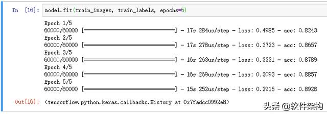
要开始训练,请调用 model.fit 方法,使模型对训练数据“拟合”:
model.fit(train_images, train_labels, epochs=5)
在模型训练期间,系统会显示损失和准确率指标。该模型在训练数据上的准确率达到约0.88(即 88%)。
8. 评估准确率接下来,比较一下模型在测试数据集上的表现:
test_loss, test_acc = model.evaluate(test_images, test_labels)
print('Test accuracy:', test_acc)
结果表明,模型在测试数据集上的准确率略低于在训练数据集上的准确率。训练准确率和测试准确率之间的这种差异表示出现过拟合。如果机器学习模型在新数据上的表现不如在训练数据上的表现,就表示出现过拟合。
9. 进行预测通过训练模型,我们可以使用它来预测某些图像。
predictions = model.predict(test_images)
在此,模型已经预测了测试集中每个图像的标签。我们来看看第一个预测:
predictions[0]
预测是10个数字的数组。这些描述了模型的"信心",即图像对应于10种不同服装中的每一种。我们可以看到哪个标签具有最高的置信度值:
np.argmax(predictions[0])
输出为:9
查看9 对应的类别 -- class_names[9],输出 Ankle boot。
接着,我们检查测试标签,看看预测是否正确:
test_labels[0]
输出为:9(说明预测结果正确)
进一步使用图表来显示全部10个类别。
首先,定义2个函数,分别为:
- plot_image 显示预测的图像;
- plot_value_array 显示针对图像预测的结果,也就是10个类别的概率值;
具体代码如下:
def plot_image(i, predictions_array, true_label, img):
predictions_array, true_label, img = predictions_array[i], true_label[i], img[i]
plt.grid(False)
plt.xticks([])
plt.yticks([])
plt.imshow(img, cmap=plt.cm.binary)
predicted_label = np.argmax(predictions_array)
if predicted_label == true_label:
color = 'blue'
else:
color = 'red'
plt.xlabel("{} {:2.0f}% ({})".format(class_names[predicted_label],
100*np.max(predictions_array),
class_names[true_label]),
color=color)
def plot_value_array(i, predictions_array, true_label):
predictions_array, true_label = predictions_array[i], true_label[i]
plt.grid(False)
plt.xticks([])
plt.yticks([])
thisplot = plt.bar(range(10), predictions_array, color="#777777")
plt.ylim([0, 1])
predicted_label = np.argmax(predictions_array)
thisplot[predicted_label].set_color('red')
thisplot[true_label].set_color('blue')
让我们看看第0个图像,预测图像和预测数组。从下图来看,预测结果正确(蓝色代码真实的类别)。
i = 0
plt.figure(figsize=(6,3))
plt.subplot(1,2,1)
plot_image(i, predictions, test_labels, test_images)
plt.subplot(1,2,2)
plot_value_array(i, predictions, test_labels)
plt.show()
让我们看看第12个图像,预测图像和预测数组。从下图来看,预测结果不正确(红色代表预测类别,蓝色代表真实类别)。
i = 12
plt.figure(figsize=(6,3))
plt.subplot(1,2,1)
plot_image(i, predictions, test_labels, test_images)
plt.subplot(1,2,2)
plot_value_array(i, predictions, test_labels)
plt.show()
让我们绘制几个图像及其预测结果。正确的预测标签是蓝色的,不正确的预测标签是红色的。该数字给出了预测标签的百分比(满分100)。请注意,即使非常自信,也可能出错。
# 绘制前X个测试图像,预测标签和真实标签
# 以蓝色显示正确的预测,红色显示不正确的预测
num_rows = 5
num_cols = 3
num_images = num_rows*num_cols
plt.figure(figsize=(2*2*num_cols, 2*num_rows))
for i in range(num_images):
plt.subplot(num_rows, 2*num_cols, 2*i 1)
plot_image(i, predictions, test_labels, test_images)
plt.subplot(num_rows, 2*num_cols, 2*i 2)
plot_value_array(i, predictions, test_labels)
plt.show()
最后,使用训练的模型对单个图像进行预测。
# 从测试数据集中获取图像
img = test_images[0]
print(img.shape)
tf.keras模型经过优化,可以一次性对批量,或者一个集合的数据进行预测。因此,即使我们使用单个图像,我们也需要将其添加到列表中:
# 将图像添加到批次中,即使它是唯一的成员。
img = (np.expand_dims(img,0))
print(img.shape)
现在来预测图像:
predictions_single = model.predict(img)
print(predictions_single)
上图输出了单个预测结果的图形化显示,比较直观。
model.predict 返回一个包含列表的列表,每个图像对应一个列表的数据。获取批次中第0个图像的预测:
prediction_result = np.argmax(predictions_single[0])
print(prediction_result)
和上一步,我们的预测结果(9)是一样的 - Ankle boot。
上述操作步骤和完整的代码,可以访问如下链接:
https://notebooks.azure.com/rickiechina/projects/pythontutorial/html/Tensorflow-Tutorial.ipynb
好啦 ... 应该感谢一下自己的坚持和努力!!!
对TensorFlow 有兴趣的同学,可以访问如下链接:
参考链接:
训练您的第一个神经网络: 基本分类
https://tensorflow.google.cn/tutorials/keras/basic_classification
zalandoresearch/fashion-mnist
https://github.com/zalandoresearch/fashion-mnist/blob/master/README.zh-CN.md
Train your first neural network: basic classification
https://www.ziiai.com/docs/tensorflow/tutorials/keras/basic_classification
,