深度学习可以捕获一个图像的内容并将其与另一个图像的风格相结合,这种技术称为神经风格迁移。但是,神经风格迁移是如何运作的呢?在这篇文章中,我们将研究神经风格迁移(NST)的基本机制。

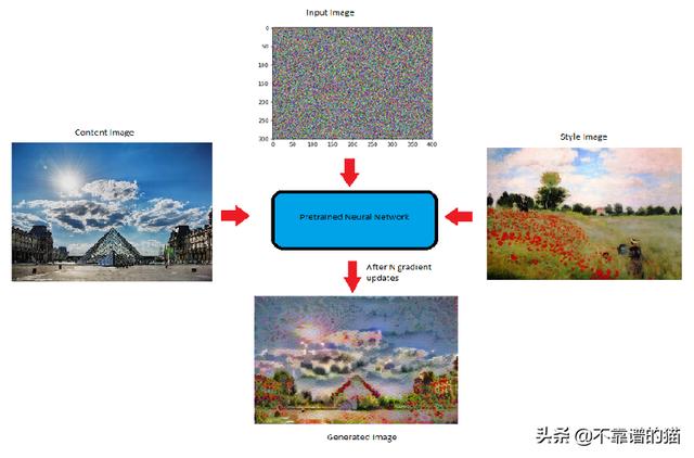
神经风格迁移概述
我们可以看到,生成的图像具有内容图像的内容和风格图像的风格。可以看出,仅通过重叠图像不能获得上述结果。我们是如何确保生成的图像具有内容图像的内容和风格图像的风格呢?
为了回答上述问题,让我们来看看卷积神经网络(CNN)究竟在学习什么。
卷积神经网络捕获到了什么
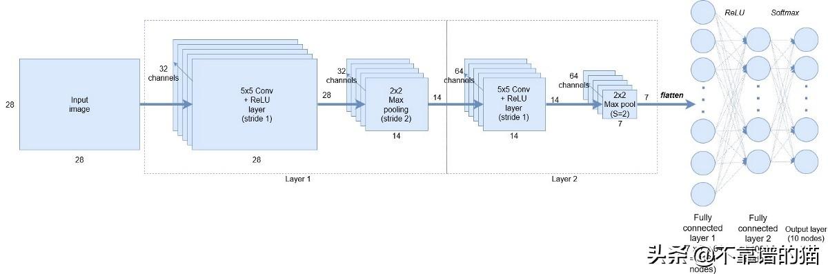
卷积神经网络的不同层
现在,在第1层使用32个filters ,网络可以捕捉简单的模式,比如直线或水平线,这对我们可能没有意义,但对网络非常重要,慢慢地,当我们到第2层,它有64个filters ,网络开始捕捉越来越复杂的特征,它可能是一张狗的脸或一辆车的轮子。这种捕获不同的简单特征和复杂特征称为特征表示。
这里需要注意的是,卷积神经网络(CNN)并不知道图像是什么,但他们学会了编码特定图像所代表的内容。卷积神经网络的这种编码特性可以帮助我们实现神经风格迁移。
卷积神经网络如何用于捕获图像的内容和风格VGG19网络用于神经风格迁移。VGG-19是一个卷积神经网络,可以对ImageNet数据集中的一百多万个图像进行训练。该网络深度为19层,并在数百万张图像上进行了训练。因此,它能够检测图像中的高级特征。
现在,CNN的这种“编码性质”是神经风格迁移的关键。首先,我们初始化一个噪声图像,它将成为我们的输出图像(G)。然后,我们计算该图像与网络中特定层(VGG网络)的内容和风格图像的相似程度。由于我们希望输出图像(G)应该具有内容图像(C)的内容和风格图像(S)的风格,因此我们计算生成的图像(G)的损失,即到相应的内容(C)和风格( S)图像的损失。
有了上述直觉,让我们将内容损失和风格损失定义为随机生成的噪声图像。
NST模型
内容损失计算内容损失意味着随机生成的噪声图像(G)与内容图像(C)的相似性。为了计算内容损失:
假设我们在一个预训练网络(VGG网络)中选择一个隐藏层(L)来计算损失。因此,设P和F为原始图像和生成的图像。其中,F[l]和P[l]分别为第l层图像的特征表示。现在,内容损失定义如下:

内容成本函数
风格损失在计算风格损失之前,让我们看看“ 图像风格 ”的含义或我们如何捕获图像风格。

层l中的不同通道或特征映射
这张图片显示了特定选定层的不同通道或特征映射或filters。现在,为了捕捉图像的风格,我们将计算这些filters之间的“相关性”,也就是这些特征映射的相似性。但是相关性是什么意思呢?
让我们借助一个例子来理解它:
上图中的前两个通道是红色和黄色。假设红色通道捕获了一些简单的特征(比如垂直线),如果这两个通道是相关的,那么当图像中有一条垂直线被红色通道检测到时,第二个通道就会产生黄色的效果。
现在,让我们看看数学上是如何计算这些相关性的。
为了计算不同filters或信道之间的相关性,我们计算两个filters激活向量之间的点积。由此获得的矩阵称为Gram矩阵。
但是我们如何知道它们是否相关呢?
如果两个filters激活之间的点积大,则说两个通道是相关的,如果它很小则是不相关的。以数学方式:
风格图像的Gram矩阵(S):
这里k '和k '表示层l的不同filters或通道。我们将其称为Gkk ' [l][S]。

用于风格图像的Gram矩阵
生成图像的Gram矩阵(G):
这里k和k'代表层L的不同filters或通道。让我们称之为Gkk'[l] [G]。

生成图像的Gram矩阵
现在,我们可以定义风格损失:
风格与生成图像的成本函数是风格图像的Gram矩阵与生成图像的Gram矩阵之差的平方。

风格成本函数
现在,让我们定义神经风格迁移的总损失。
总损失函数:总是内容和风格图像的成本之和。在数学上,它可以表示为:

神经风格迁移的总损失函数
您可能已经注意到上述等式中的Alpha和beta。它们分别用于衡量内容成本和风格成本。通常,它们在生成的输出图像中定义每个成本的权重。
一旦计算出损失,就可以使用反向传播使这种损失最小化,反向传播又将我们随机生成的图像优化为有意义的艺术品。
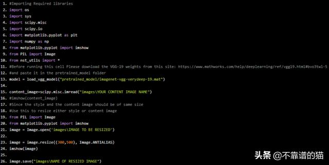
使用tensorflow实现神经风格迁移Python示例代码:#Importing Required libraries import os import sys import scipy.misc import scipy.io import matplotlib.pyplot as plt import numpy as np from matplotlib.pyplot import imshow from PIL import Image from nst_utils import * #Before running this cell Please download the VGG-19 weights from this site: https://www.mathworks.com/help/deeplearning/ref/vgg19.html#bvo3tw1-5 #and paste it in the pretrained_model folder model = load_vgg_model("pretrained_model/imagenet-vgg-verydeep-19.mat") content_image=scipy.misc.imread("images\YOUR CONTENT IMAGE NAME") #imshow(content_image) #Since the style and the content image should be of same size #Use this to resize either style or content image from PIL import Image from matplotlib.pyplot import imshow image = Image.open('images\IMAGE TO BE RESIZED') image = image.resize((300,500), Image.ANTIALIAS) imshow(image) image.save("images\NAME OF RESIZED IMAGE")

style_image=scipy.misc.imread("images\style1.jpg") imshow(style_image)

辅助函数
def compute_content_cost(a_C,a_G): m,n_H,n_W,n_C=a_G.get_shape().as_list() a_C_unrolled=tf.transpose(a_C) a_G_unrolled=tf.transpose(a_G) #Content_cost: J_content=(1/(4 * n_H * n_W * n_C)) * tf.reduce_sum(tf.pow((a_C_unrolled - a_G_unrolled),2)) return J_content def gram_matrix(A): GA=tf.matmul(A,tf.transpose(A)) return GA def compute_layer_style_cost(a_S,a_G): m,n_H,n_W,n_C=a_G.get_shape().as_list() #Reshape: a_S=tf.transpose(tf.reshape(a_S,[n_H * n_W, n_C])) a_G=tf.transpose(tf.reshape(a_G,[n_H * n_W, n_C])) #Gram matrix: GS=gram_matrix(a_S) GG=gram_matrix(a_G) #Cost: J_style=(1/(4 * (n_C)**2 * (n_H * n_W)**2)) * tf.reduce_sum(tf.pow((GS - GG),2)) return J_style STYLE_LAYERS = [ ('conv1_1', 0.2), ('conv2_1', 0.2), ('conv3_1', 0.2), ('conv4_1', 0.2), ('conv5_1', 0.2)] def compute_style_cost(model,STYLE_LAYERS): J_style = 0 for layer_name, coeff in STYLE_LAYERS: # Select the output tensor of the currently selected layer out = model[layer_name] # Set a_S to be the hidden layer activation from the layer we have selected, by running the session on out a_S = sess.run(out) # Set a_G to be the hidden layer activation from same layer. Here, a_G references model[layer_name] # and isn't evaluated yet. Later in the code, we'll assign the image G as the model input, so that # when we run the session, this will be the activations drawn from the appropriate layer, with G as input. a_G = out # Compute style_cost for the current layer J_style_layer = compute_layer_style_cost(a_S, a_G) # Add coeff * J_style_layer of this layer to overall style cost J_style = coeff * J_style_layer return J_style def total_cost(J_content, J_style, alpha = 10, beta = 40): J = alpha * J_content beta * J_style return J

优化及神经网络模型
tf.reset_default_graph() sess=tf.InteractiveSession() content_image=scipy.misc.imread("images\YOUR CONTENT IMAGE") content_image = reshape_and_normalize_image(content_image) style_image = scipy.misc.imread("images/YOUR STYLE IMAGE") style_image = reshape_and_normalize_image(style_image) #Generating a noisy image generated_image = generate_noise_image(content_image) imshow(generated_image[0]) model = load_vgg_model("pretrained_model/imagenet-vgg-verydeep-19.mat") sess.run(model['input'].assign(content_image)) out=model['conv4_2'] a_C = sess.run(out) a_G=out J_content = compute_content_cost(a_C, a_G) sess.run(model['input'].assign(style_image)) # Compute the style cost J_style = compute_style_cost(model, STYLE_LAYERS) J = total_cost(J_content, J_style, alpha = 10, beta = 40) # define optimizer (1 line) optimizer = tf.train.AdamOptimizer(2.0) # define train_step (1 line) train_step = optimizer.minimize(J) def model_nn(sess, input_image, num_iterations = 1000): # Initialize global variables (you need to run the session on the initializer) sess.run(tf.global_variables_initializer()) # Run the noisy input image (initial generated image) through the model. Use assign(). sess.run(model['input'].assign(input_image)) for i in range(num_iterations): # Run the session on the train_step to minimize the total cost sess.run(train_step) # Compute the generated image by running the session on the current model['input'] generated_image = sess.run(model['input']) # Print every 20 iteration. if i == 0: Jt, Jc, Js = sess.run([J, J_content, J_style]) print("Iteration " str(i) " :") print("total cost = " str(Jt)) print("content cost = " str(Jc)) print("style cost = " str(Js)) # save current generated image in the "/output" directory save_image("output/" str(i) ".png", generated_image) # save last generated image save_image('output/generated_image.jpg', generated_image) return generated_image model_nn(sess, generated_image)


在这篇文章中,我们深入研究了神经风格迁移的工作原理。我们还讨论了NST背后的数学。
,