r语言的回归模型t值怎么求（R语言主成分分析）

使用R语言为PCA散点图加置信区间的方法，我知道的有三种，分别是使用ggplot2,ggord,ggfortify三个包去绘制。后面两个R包是基于ggplot2的快捷返方法。

现在拿一组数据集为例，使用先R中的prcomp()基础函数完成主成分分析

查看数据类型，每一列代表一个样本，每一行代表一个基因（变量） > head(a,3) X1_untreated X2_untreated X3_untreated X4_untreated X1_Dex X2_Dex ENSG00000223972 -2.089725 -2.090478 -2.090475 -2.089265 -2.079351 -2.087724 ENSG00000227232 6.760110 6.892673 6.346646 6.739761 6.450597 6.749787 ENSG00000243485 0.000000 0.000000 0.000000 0.000000 0.000000 0.000000 X3_Dex X4_Dex ENSG00000223972 -2.091304 -2.089408 ENSG00000227232 6.623112 6.524621 ENSG00000243485 0.000000 0.000000 b <- t(a)#PCA分析需要将表达矩阵转置 -----------------标准化处理-------------- R函数：scale(data, center=T/F, scale=T/F)或者scale(data) 参数：center (中心化)将数据减去均值，默认为T 参数：scale (标准化)在中心化后的数据基础上再除以数据的标准差,默认值F,建议改为T c <- prcomp(b[ , which(apply(data, 2, var) != 0)], scale=TRUE) summary(c) 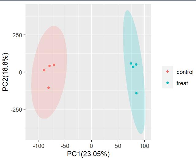可以看到pc1方差的解释率达23.05%，pc2的方差的解释率达18.8%，等等 Importance of components: PC1 PC2 PC3 PC4 PC5 PC6 PC7 PC8 Standard deviation 86.1425 77.7838 71.9321 64.5281 59.7924 54.48867 53.27203 3.021e-12 Proportion of Variance 0.2305 0.1880 0.1607 0.1293 0.1111 0.09223 0.08816 0.000e 00 Cumulative Proportion 0.2305 0.4185 0.5792 0.7086 0.8196 0.91184 1.00000 1.000e 00 >

提取不同记录的PC1-PC8数值，即点的横纵坐标值 dt = c$x > head(dt,3) PC1 PC2 PC3 PC4 PC5 PC6 PC7 X1_untreated -70.89354 47.84633 -93.91127 3.457347 -32.08983 -72.516671 60.80422 X2_untreated -89.78212 14.29189 61.29232 -102.245406 -39.00539 59.352006 21.05424 X3_untreated -81.40448 -105.32841 -15.33420 19.990771 107.24132 9.986499 4.28529 PC8 X1_untreated 2.802701e-12 X2_untreated 2.715383e-12 X3_untreated 2.618101e-12 condition condition 1 control 2 control 3 control 4 control 5 treat 6 treat 7 treat 8 treat 将condition列添加到dt中 dt = cbind(dt,condition) > head(dt,3) PC1 PC2 PC3 PC4 PC5 PC6 PC7 X1_untreated -70.89354 47.84633 -93.91127 3.457347 -32.08983 -72.516671 60.80422 X2_untreated -89.78212 14.29189 61.29232 -102.245406 -39.00539 59.352006 21.05424 X3_untreated -81.40448 -105.32841 -15.33420 19.990771 107.24132 9.986499 4.28529 PC8 condition X1_untreated 2.802701e-12 control X2_untreated 2.715383e-12 control X3_untreated 2.618101e-12 control 生成坐标轴标题 summ = summary(c) xlab = paste0("PC1(",round(summ$importance[2,1]*100,2),"%)") ylab = paste0("PC2(",round(summ$importance[2,2]*100,2),"%)") 载入ggplot2包 library(ggplot2) ggplot(data = dt,aes(x=PC1,y= PC2,color=condition)) stat_ellipse(aes(fill=condition),type="norm",geom="polygon",alpha=0.2,color=NA) geom_point() labs(x=xlab,y=ylab,color="") guides(fill=F)